Temporal Rate Rescaling
PalantiR uses a rescaling strategy to simulate smooth transitions in temporal heterogeneity simulations. Temporal heterogeneity simulations have a “switch point” from one substitution model to another. This can correspond to a fitness shift or a population size change.
The idea is to continuously rescale the substitution rate matrix until the equilibrium distribution of the rescaled rates matrix matches that of the new matrix we switch into.
Example
Rescaling
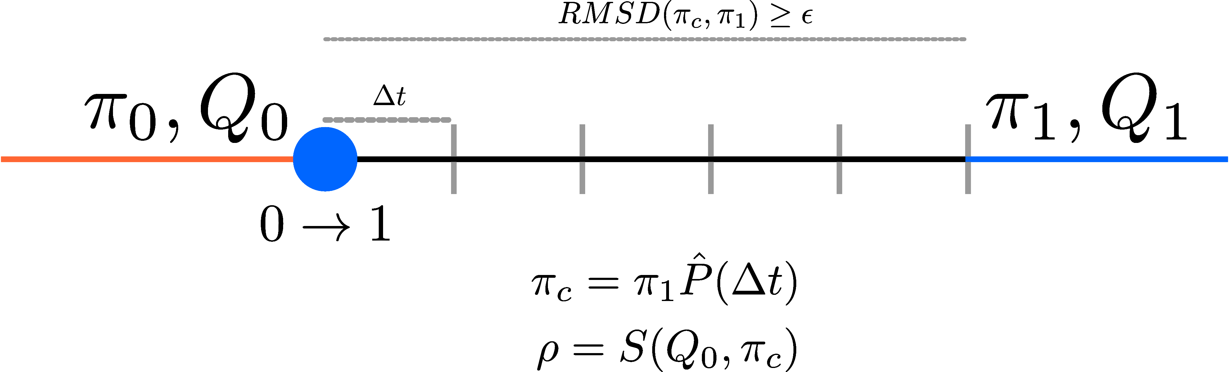
The figure shows a branch on which a switch occurs from substitution model 0 to to substitution model 1. Model 0 has a switching rates matrix Q0 and an equilibrium distribution π0. The branch segment where model 0 applies is represented by an orange line.
The switch into model 1 is represented by a blue circle. The branch is now segmented into small sections of length Δt. We now calculate a rescaled version of Q and π for each of the branch segments.
Rescaling
The idea is to calculate an empirical π for a short branch segment, given Δt.
For a small t, we can approximate transition probability P as P ≈ Q⋅Δt + I.
We then estimate the empirical π for the current branch segment as π⋅P.
Using the current estimate of π, we now want to calculate a scaling factor ρ, which will be used to rescale the current substitution rate matrix. The scaling function S is discussed in more details in [[scaling|Rate Matrix Scaling]].
The rescaled matrix Q is now used to simulate substitutions for the current branch segment.
The rescaling procedure is applied until the current π is within an acceptable range of the π for next model. Once the RMSD between the two equilibrium vectors is within user-specified bound ε, the rescaling is stopped. At this point, the simulation continues with substitution rate Q1 and equilibrium distribution π1, corresponding to the model 1 (blue branch segment).
de Koning Lab. 2016-2017 lab.jasondk.io